南京大学唐朝生教授团队:基于电阻率层析成像的微生物诱导碳酸钙沉淀时空分布重构

摘要

主要图表

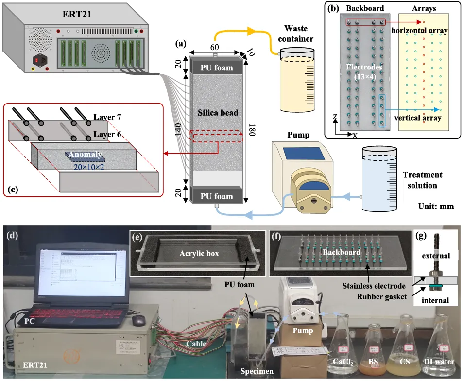
Fig. 1. Sketch and photo of the experimental setup. (a) Silica beads were packed into the acrylic box (60 × 10 × 180 mm). (b) Fifty-two stainless electrodes were installed on the backboard of the box, which was used for the electrical conductivity measurement and tomography. (c) Specimens B2 and B3 have the permeability anomaly at the center of the box, which is an acrylic sheet and a polyurethane (PU) foam, respectively. (d)-(g) Photos of the electrical measurement system (ERT21), acrylic box, electrode backboard, and stainless electrodes.

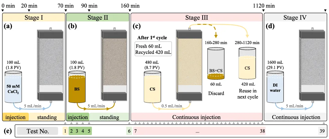
Fig. 2. Procedure of MICP treatment in one cycle (a)-(d) and the correlated electrical monitoring scheme (e). The specimen has a pore volume (PV) of 55 cm³ .

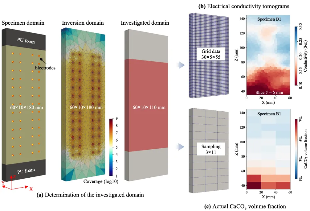
Fig. 3. Determination of the investigated domain.

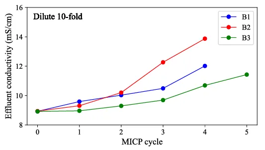
Fig. 4. Effluent conductivity (cementation solution conductivity) after each MICP cycle in the three specimens (B1, B2, and B3). Since the effluents were recycled for the next MICP cycle (see Fig. 2c), the increase in effluent conductivity can indicate the increase in ion concentration and the progress of mineralization reactions.

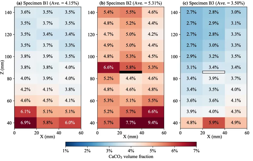
Fig. 5. The actual CaCO₃ volume fraction after all MICP treatment.

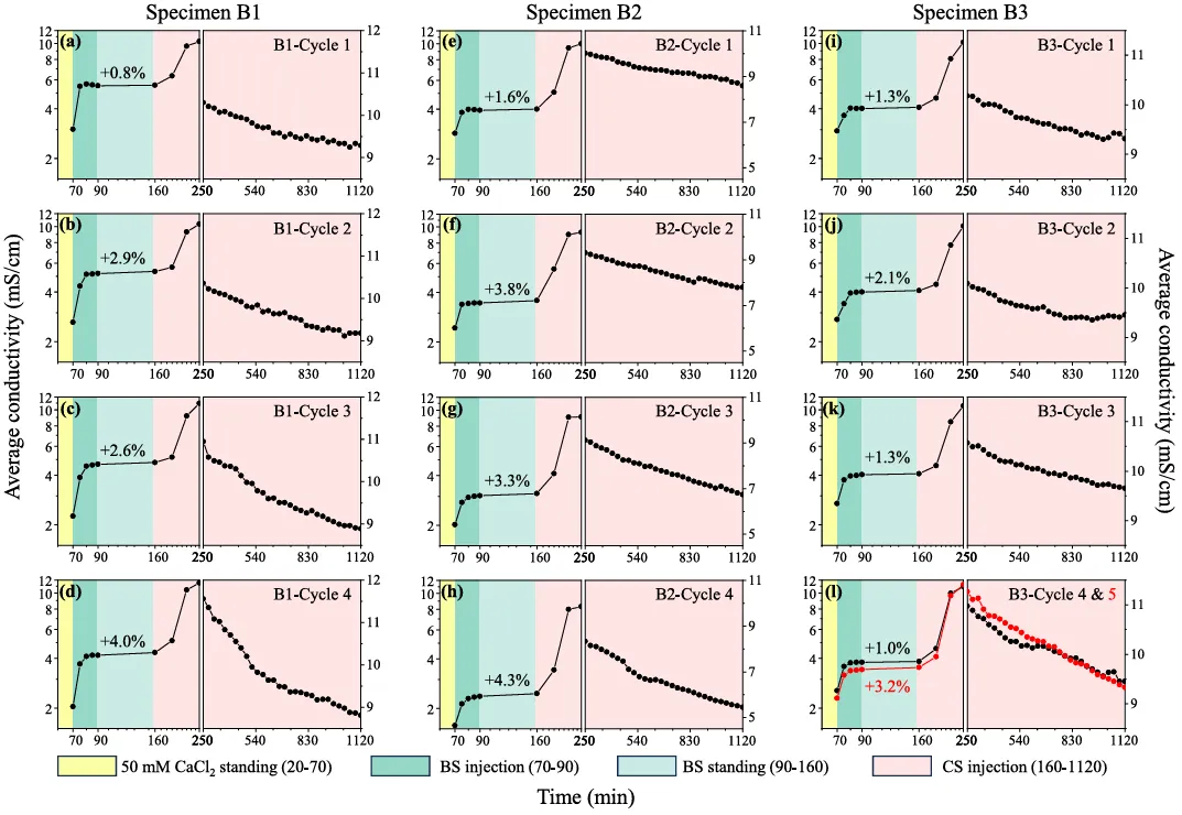
Fig. 6. The evolution of average specimen conductivity with time during each treatment cycle.

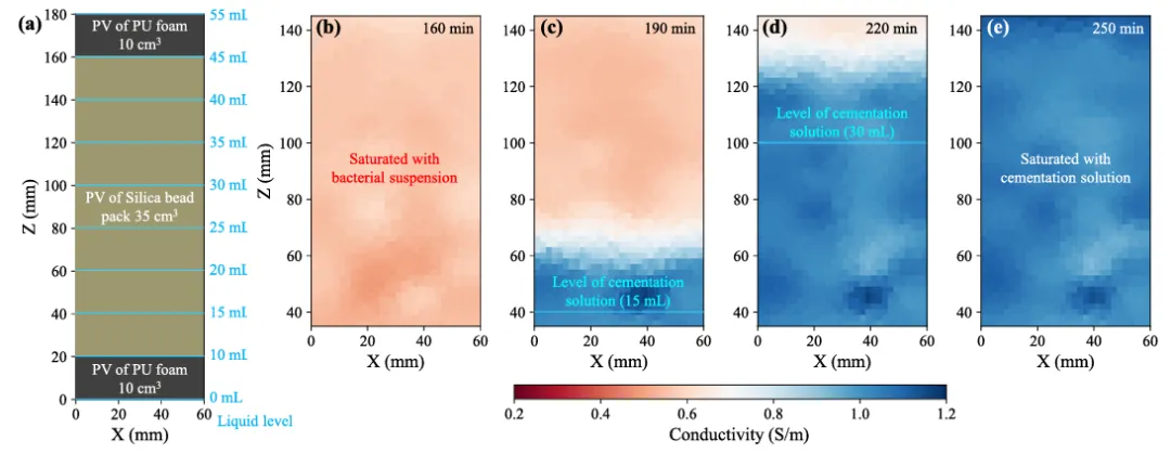
Fig. 7. The liquid level in the specimen with injected fluids of different volumes (a) and conductivity tomograms during the cementation solution (CS) injection (b)- (d). The low conductivity zone corresponded to the specimen saturated with bacterial suspension (BS), while the high conductivity zone corresponded to the specimen saturated with CS. The injection of CS started at 160 min with a rate of 0.5 mL/min. 15 mL of CS was injected at 190 min, and 30 mL of CS was injected at 220 min. These two levels of CS are indicated by light-blue solid lines in (c) and (d). (For interpretation of the references to colour in this figure legend, the reader is referred to the web version of this article.)

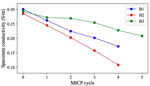
Fig. 8. Specimen average conductivity after each MICP treatment cycle.

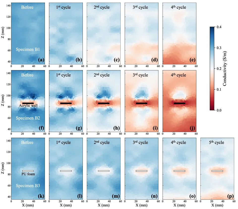
Fig. 9. Electrical conductivity tomograms before and after each MICP treatment cycle.

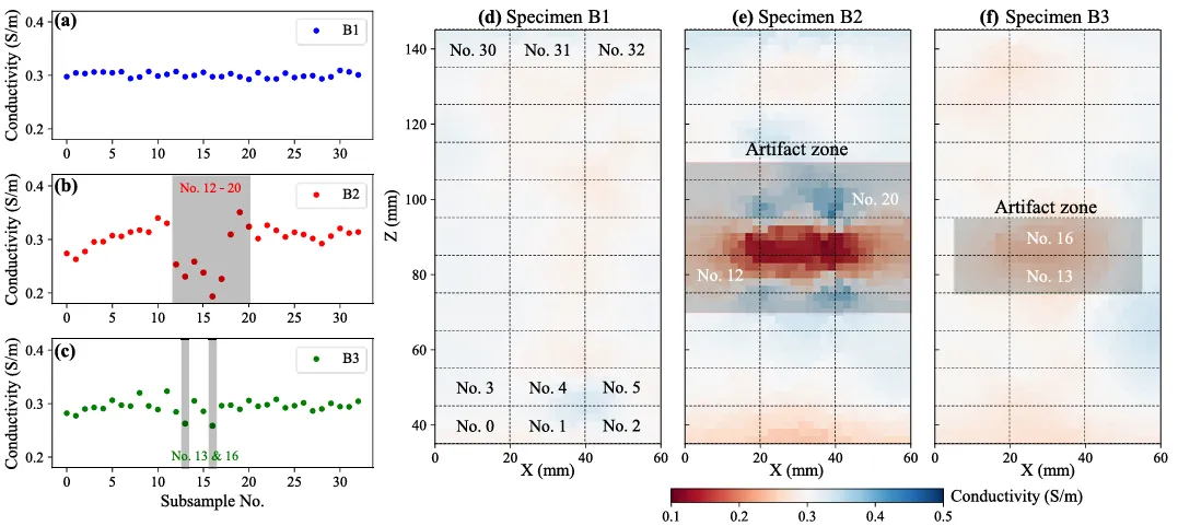
Fig. 10. Resampling the interpreted conductivity model before MICP treatment.

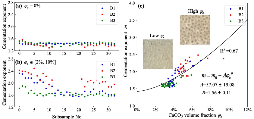
Fig. 11. . Cementation exponent m of resampled silica beads pack before and after the MICP treatment (a-b).(c) The cementation exponent m and CaCO₃ volume fraction φc of the cemented silica beads were fitted with Eq. 9.

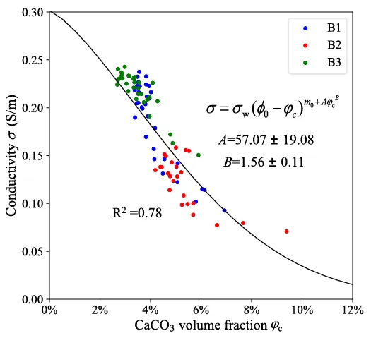
Fig. 12. Petrophysical model between electrical conductivity and CaCO₃ volume fraction in MICP-treated silica bead pack.

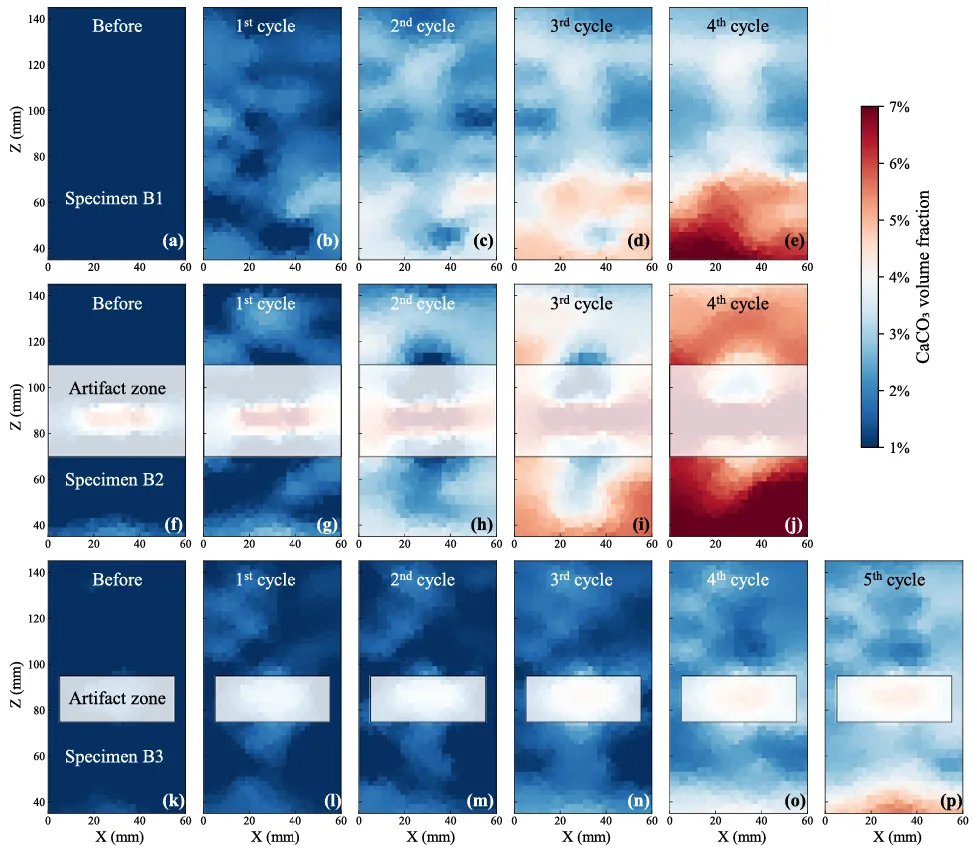
Fig. 13. Spatiotemporal evolution of the volume fraction of CaCO₃ for the three specimens after each MICP treatment cycle.

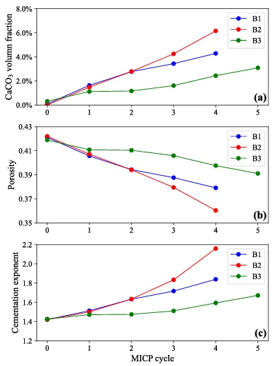
Fig. 14. Evolution of the average CaCO₃ volume fraction φc, porosity ϕ, and cementation exponent m of the silica bead packs after each MICP cycle. φc was estimated using the average electrical conductivity after each MICP cycle based on the proposed petrophysical model (Eq. 10). ϕ and m can be determined based on Eqs. 5 and 9.

研究结论